Why you should know about the Gamma distribution

Dec 02, 2016

I’ve been staring at exponentially distributed data in various forms for at least the last ten years. In my previous job, I spent a lot of time with the statistics of VoIP phone calls, trying to understand what’s “normal”, and what are symptoms of system pathologies, or even the actions of fraudsters in the telephony networks. In approaching this subject long ago, I had not yet studied queuing theory, but I had a lot of experience with Poisson processes in experimental high energy physics. This meant that as I learned I had many wonderful eureka! moments. One of these moments was when I learned that the sum of exponentially distributed variables has a gamma distribution. I often find that people I mention this to, people in systems, and even often in machine learning, are unfamiliar with this fact, or why it would be useful to know.

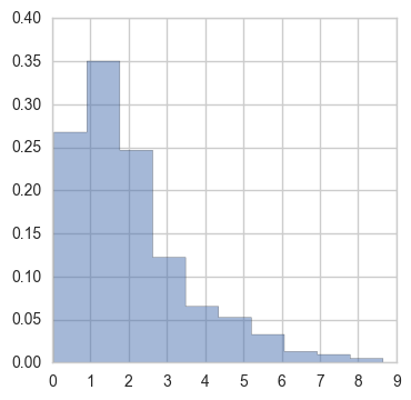
In fact, this is a very helpful thing to know when looking at the distributions of many things you measure in systems, for you often see a long-tailed distribution where the mode is shifted to the right, relative to where the exponential would start. This is what scipy.stats.gamma.rvs(1.99, size=1000) looks like:

The reason this is really helpful to think about is you often find yourself looking at the length of the intervals it takes for things to complete:

the time it takes IO requests to complete
the time it takes a program to run
the amount of time a lock is held
the time it takes to resolve a ticket

One way to think about what is happening behind the scenes is that you are looking at many different system components taking part, and each taking some time to do it’s job. What you see then when you wait for the entire completion is then the sum of many individual component times. When we model the individual times as exponentially distributed, we then should expect that what we measure should follow a gamma-like distribution. When reasoning about systems, looking at the distribution of times tells you a lot about what’s happening. 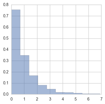When the data looks exponentially-distributed, i.e. the mode is all the way to the left (scipy.stats.expon.rvs(size=1000))

An Exponential — A Exponential distribution from Scipy

then you really have one dominant process contributing to the completion time. Instead, the more you see the mode shifted to the right, the more you can reason that there are a number of processes of equal contribution. This is a useful way to reason about systems.

As I said, learning that the sums of exponentials was distributed as gamma was a neat and useful eureka! moment. However, until recently, I missed an extremely important related fact. All of this came about when I found a need to perform a computationally efficient test to determine if the distributions two sets of exponentially distributed data differed. This lead to another eureka! moment that I will describe below.

The Gamma distribution

Most folks are familiar with the gamma function, which extends the factorial function to complex numbers with positive real part:

\begin{align} \Gamma(z) &= \int_0^{\infty} t^{z-1} e^{-t} dt\\ &= (z-1)!,\, z \in \mathbb{C}, Re(z) > 0.\\ \end{align}

But fewer people seem to know about the gamma distribution, which is defined to be

\begin{align} G(k, \theta) = \frac{1}{\Gamma(k)\,\theta^k} x^{k-1} e^{-x/\theta}\\ \end{align}

where $k$ is the scale and $\theta$ is the shape. The gamma distribution can be seen as a generalization of two other commonly encountered distributions, $\chi_k^2$ and $Exp(\lambda)$:

\begin{align} G(k/2, 2) &= \frac{1}{\Gamma(k/2)\,2^{k/2}} x^{k/2-1} e^{-x/2}\\ &= \chi_k^2\\ G(1, \theta) &= \frac{1}{\theta} e^{-x/\theta}\\ &= Exp(\lambda = 1/\theta)\\ \end{align}

The generality of the gamma goes even further. Not only is it is it’s own conjugate prior, it’s the conjugate prior for a large number of important distributions: Poisson, Normal, Pareto, Log-normal, Exponential.

But let’s get back to proving some neat things about this distribution. Before we can start, we will need one additional piece of machinery. In The Coupon Collector, I showed a useful application for probability generating functions (PGFs), which, to review, are

\begin{align} G(z) &= \sum_0^\infty f_k z^k\\ &= \mathbb{E} \left[ z^k \right]\\ \end{align}

under the discrete distribution $f_k$. A handy generalization of PGFs is create moment generating functions (MGFs), by taking

\begin{align} M_X (t) &= G_X(e^t)\\ &= \mathbb{E}\left[ e^{tX}\right].\\ \end{align}

MGFs have all the nice manipulation tricks of PGFs, have even nicer derivative-taking properties than PGFs, and work for both continuous and discrete distributions. And as long as we are careful about integrating over the support of $f(x)$, they also have the very interesting expression as

\begin{align} M_X (t) &= \int_{-\infty}^{\infty} e^{tx} f(x) dx\\ \end{align}

which might be recognized as the two-sided Laplace transform of the distribution $f(x)$. Previously, we saw that one answer to “why did I do all of these contortions on PGFs” was that taking derivatives gave us nice and easy ways to calculate the mean, variance, etc. The MGFs also give us these as the moments of the distribution. But the definition above provides us another trick, namely that if we are careful about the the above definition, we can take the inverse Laplace transform of a MGF to derive a distribution. Deriving distributions can be trickery, so this is a nice tool to have in the box. We may return to calculating $\mathcal{L}^{-1}\left\{ M_X(t) \right\}$ in another post.

So, what is the MGF for the gamma distribution? By definition we have

\begin{align} M_{G(k,\theta)}(t) &= \mathbb{E} \left[ e^{tx} \right]\\ &= \int_0^\infty e^{tx} G\left(x \vert k,\theta\right) dx\\ &= \frac{1}{\Gamma(k)\, \theta^k} \int_0^\infty x^{k-1} e^{-x\left(1/\theta - t\right)} dx, \, t \theta < 1\\ &= \frac{1}{\Gamma(k)\, \theta^k\, (1/\theta - t)^k} \int_0^\infty x^{k-1} e^{-x} dx\\ &= \frac{1}{\Gamma(k)\, \theta^k\, (1/\theta - t)^k} \Gamma(k)\\ &= (1 - \theta t)^{-k}\\ \end{align}

With that we are ready to derive the first result we need. Assume we have a set of IID random variables $X_i \sim G(a_i, \theta)$ for some arbitrary $a_i$ and fixed $\theta$. Let’s consider the sum of these variables $S_n = \sum_n X_i$. Now looking at the MGF,

\begin{align} M_{S_n}(t) &= \mathbb{E}\left[ e^{t S_n} \right]\\ &= \mathbb{E}\left[ \prod_{i=1}^n e^{t x_i} \right]\\ &= \prod_{i=1}^n \mathbb{E}\left[e^{t x_i} \right]\\ &= \prod_{i=1}^n (1- \theta t)^{-a_i} \\ &= (1- \theta t)^{-\sum a_i} \\ &= M_{G(\sum a_i, \theta)}.\\ \end{align}

In the third step we have used the independence of the $X_i$ to move the product outside of the expectation. Looking at the last line, we identify the result as the MGF for $G(\sum a_i, \theta)$. We then conclude that

\begin{align} S_n &\sim G\left(\sum_{i=1}^n a_i, \theta\right).\\ \end{align}

Which is to say that the sum of gamma distributed variables $X_i$ of scales $a_i$ is distributed as a gamma of scale $\sum a_i$. This result carries my original eureka! moment, namely that if $X_i \sim Exp(\lambda = 1/\theta) = G(1, \theta)$, then

$$ S_n = \sum_n X_i \sim G\left(n, \theta\right). $$

Incidentally this also means that if $X_i \sim \chi^2_{n_i} = G(n_i/2, 2)$, then the sum over those variables

$$ S_n = \sum_n X_i \sim G \left( 1/2 \sum n_i, 2\right) = \chi^2_{\sum n_i} $$

A similar calculation to the above gives us another property of $G(k,\theta)$, namely that if If $X \sim G(k, \theta)$, then

\begin{align} cX &\sim G(k, c \theta).\\ \end{align}

This means that if $X_i \sim Exp(\lambda = 1/ \theta)$,

\begin{align} \frac{2}{\theta} S_n \sim G(n, 2) = \chi^2_{2n}.\\ \end{align}

When I first saw this, I thought it was just amazing. Now let me explain why.

Making sense of program run-times

As mentioned above, one of my current projects started all of this thinking. I have been working on a simple library to do performance-based regression testing, which I will talk more about that in a later post, but for now, I present below some of the benchmarking data that I have been working with. Each histogram is labeled by a number which is $k = log N$ of the total input size of the code being tested. Specifically, I am benchmarking a library that uses Intel SSE4.2 specialized instructions to calculate crc32c checksums.

Program runtimes for crc32c checksum calculation using Intel SSE4.2 instructions. Plots are labeled by input size.

There are a ton of interesting details going on that I will discuss later, but it should be clear that for each $k$, every time I make these measurements I will get different looking histograms. They could be different because something changed in the code. Or, they could be different just because we are dealing with random variables. All I really want to know is if something has changed in the code, assembly, or even underlying architecture. This will allow me to fail the regression test with some meaningful statistical confidence. For profiling reasons, I might be interested in the parameters, but primarily I need to detect changes.

The usual way to deal with this kind of data situation is to take large number of samples $n_k$. But because my testing library needs to run very fast, taking a large number of sample is unacceptable since the total test run time is proportional to the number of samples collected. I need to test my histogram sets against each other using as few total $\sum_k n_k$ as possible. Mainly this is because in my experience, the probability of a test being manually disabled is proportional to the time it takes to run the test. We need a system that no one every think about disabling. Also, my personal development style is to run the all dependent test-suites at every compile, not just at every check-in. So, it needs to be fast.

This is a good time to point out that by now most people looking at data like these have gone ahead and assumed the values are Gaussian and have computed a $\mu$ (and probably a $\sigma$). It is a happy or sad (depending on your perspective) fact that the MLE for $\lambda$ for an exponential distribution is

$$ \hat{\lambda} = \frac{n}{\sum_i x_i} = \frac{1}{\bar{x}} $$

For me it’s sad because it lets people get away with taking averages of data like the above and waving their hands around that they are quote-un-quote Gaussian. But I digress.

For my own purposes, what I need is a meaningful statistical test that can help me detect a change in the code. This brings me to why I got excited when I learned that

$$ \frac{2}{\theta} S_n \sim G(n, 2) = \chi^2_{2n}. $$

Seeing a $\chi^2$ gives me an idea. If $X_1 \sim \chi^2_{n_1}$ and $X_2 \sim \chi^2_{n_2}$, then

$$ U = \frac{X_1 / n_1}{X_2 / n_2} \sim F(2 n_1, 2 n_2) $$

where $F$ is the $F$-distribution. In our case,

\begin{align} U &= \frac{\frac{2 S_{n'}}{\theta' n'}}{\frac{2 S_n}{\theta n}}\\ &= \frac{\theta}{\theta'} \frac{\bar{x}'}{\bar{x}}\\ \end{align}

is distributed in $F(2n',2n)$. Thus we test $H_0$ vs $H_1$:

\begin{align} H_0 &: \theta/\theta' = 1\\ H_1 &: \theta/\theta' \neq 1.\\ \end{align}

Using tables or evaluation of $F$, we can then derive a two sided $p$-value and also confidence bounds. The $p$-value will be found from

$$ p = 2 P(F(2n',2n) < U) $$

whereas the confidence $95%$ interval is

$$ P\left(\frac{U}{T_{0.975}} < \theta/\theta' < \frac{U}{T_{0.025}} \right) = 0.95 $$

where $T_{0.975}$ and $T_{0.025}$ are the $m$ quantiles on $F(2n', 2n)$.

That’s it for now. I’ll explain how I’m using this in another post.

Why you should know about the Gamma distribution

The Gamma distribution

Making sense of program run-times

Read more in Systems

Read more in …

Reach me